A while back I decided to look into player consistency, but after doing initial calculations, I never went any further. After Namita Nandakumar's VANHAC presentation on consistency, I decided to go back, refine my old work, and release the results. Namita's methodology is likely much more statistically relevant and meaningful, but nonetheless, I use a different approach that I think is worth sharing.
The methodology I adopted was taken from this article on Nylon Calculus on NBA player consistency written by Hal Brown. This consistency metric gets the normalized variance of a player's performance for a given metric. In this post, I will be calculating the consistency of a player's game score (GS) in individual seasons, from 2007-08 to 2015-16, using the data provided at the bottom of the linked game score article. I also have a folder with my code + better resolution graphs + data at the bottom of the article if you'd like to check it out.
Calculation
This calculation begins by taking the absolute value of the z-score of every game at the individual player level.
ex. Using Sam Gagner's 2011-12 season. Gagner's mean GS = 0.59 with a standard deviation GS = 1.12
In his stellar 8 point game against Chicago, he registered a GS of 7.1.
That same season, Gagner had a GS of -1.0 on 12/15/2011. This would be calculated as:
Consistency (Con) is now calculated as the average of the absolute values of the z-scores from each game.
A lower z-score is assigned to games closer to a player's mean performance, while a higher z-score is assigned to games further from a player's mean. As such, a lower consistency score means a player is more consistent, and vice versa.
Absolute values are used to show consistency across good and bad games. For example, if a player participates in only two games and has GS of 2 and -2, the z-scores would be 0.71 and -0.71, and Con would be 0, meaning the player is perfectly consistent. We know this isn't true, as the player had two different performances. Using absolute values, this player now has a Con of 0.71, which reflects the varying performances of this player.
This calculation was done for every skater and goalie from 2007-08 to 2015-16.
Skater Results
I first looked at the relationship between GS per 60 and consistency in skaters, plotted below with some key points labeled. The plot is split into four labeled quadrants, with horizontal and vertical lines representing the league averages for each stat- Con = 0.78, GS/60 = 1.69.
There is a slight relationship (r^2 = 0.10), suggesting that consistency is not completely independent of talent level. In fact, when viewing the four quadrant's counts,

we see that a majority of players are either consistently bad or inconsistently good. This logically makes sense, as bad players generally don't have the capability to have extreme performances, while good players see their performances fluctuate much more because of the infrequency of goals. With that said, it appears very difficult to consistently perform at an elite level for an entire season. Overall, this relationship is not too significant, and consistency seems to perform as intended, independent of talent level.
I then chose to look into several individual seasons, to see how the player's GS distribution matched up with their consistency scores. The most consistent player in this dataset, Andre Roy, played under ten minutes in every game and only registered a GS of greater than 0.5 in 5 of his 63 games and a GS of less than -0.5 once. He performed with very little impact on the game (as measured by GS) at an unbelievably consistent rate. Dubinsky, on the other hand, was the most inconsistent player of this data, having an interesting bimodal distribution, showing he frequently had performances away from his mean. The next two players, Staal and Nash, have very similar GS/60 values but are on opposite ends for consistency. Staal's distribution shows he had many solid games, but very few great and bad games, which I'd say falls in line with his overall reputation. Nash follows a similar distribution as Dubinsky, showing his inconsistency, which I'd argue also lines up with his reputation. In the next plots, I chose Malkin to get an idea of what an average player's consistency distribution looks like, and Ovechkin to view how the best season in this data was distributed.

To get a better idea of how these distributions are calculated and converted to consistency, I plotted the same players with their absolute value z_score distributions. In these plots, we can see how the players' performances differ from their means (zero), and as the plot's peak (and entire distribution) shifts further from zero the player gets more inconsistent.

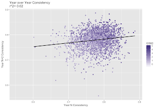
To test whether consistency is an innate skill, I looked at its year over year repeatabilities. There is no significant relationship across seasons, which agrees with Namita's consistency calculations. I'd attribute the slight positive slope to the fact that the "consistently bad" players are overall unlikely to change roles and thus remain in their position. This relationship is very weak, however, and even when filtering by player quality the r^2 stays very close to 0.

Stealing Namita's graph of consistency amongst top players, I made my own version. This shows the top 20 players in terms of overall game score over the time period being used. When plotted against league average consistency, we see that as with the first graph, elite players are typically inconsistent, simply because the most impactful events occur infrequently. In this plot, some players do appear to have a "center", which goes against the repeatability tests, but even in randomly distributed data points will cluster, and as mentioned above filtering by performance didn't change the results. Otherwise, the graph acts as a fun way to compare some of the top talents.


The methodology I adopted was taken from this article on Nylon Calculus on NBA player consistency written by Hal Brown. This consistency metric gets the normalized variance of a player's performance for a given metric. In this post, I will be calculating the consistency of a player's game score (GS) in individual seasons, from 2007-08 to 2015-16, using the data provided at the bottom of the linked game score article. I also have a folder with my code + better resolution graphs + data at the bottom of the article if you'd like to check it out.
Calculation
This calculation begins by taking the absolute value of the z-score of every game at the individual player level.
| Z | = | (X-𝜇)/𝜎 | = | (individual game GS - mean of all games GS) / (standard deviation of all games GS) |
In his stellar 8 point game against Chicago, he registered a GS of 7.1.
| Z | = | (7.1-0.59)/1.12 | = 5.81
That same season, Gagner had a GS of -1.0 on 12/15/2011. This would be calculated as:
| Z | = | (-1-0.59)/1.12 | = 1.42
A lower z-score is assigned to games closer to a player's mean performance, while a higher z-score is assigned to games further from a player's mean. As such, a lower consistency score means a player is more consistent, and vice versa.
Absolute values are used to show consistency across good and bad games. For example, if a player participates in only two games and has GS of 2 and -2, the z-scores would be 0.71 and -0.71, and Con would be 0, meaning the player is perfectly consistent. We know this isn't true, as the player had two different performances. Using absolute values, this player now has a Con of 0.71, which reflects the varying performances of this player.
This calculation was done for every skater and goalie from 2007-08 to 2015-16.
Skater Results
I first looked at the relationship between GS per 60 and consistency in skaters, plotted below with some key points labeled. The plot is split into four labeled quadrants, with horizontal and vertical lines representing the league averages for each stat- Con = 0.78, GS/60 = 1.69.
There is a slight relationship (r^2 = 0.10), suggesting that consistency is not completely independent of talent level. In fact, when viewing the four quadrant's counts,
Bad | Good
Inconsistent 1126 | 1497
Consistent 1595 | 743

we see that a majority of players are either consistently bad or inconsistently good. This logically makes sense, as bad players generally don't have the capability to have extreme performances, while good players see their performances fluctuate much more because of the infrequency of goals. With that said, it appears very difficult to consistently perform at an elite level for an entire season. Overall, this relationship is not too significant, and consistency seems to perform as intended, independent of talent level.
I then chose to look into several individual seasons, to see how the player's GS distribution matched up with their consistency scores. The most consistent player in this dataset, Andre Roy, played under ten minutes in every game and only registered a GS of greater than 0.5 in 5 of his 63 games and a GS of less than -0.5 once. He performed with very little impact on the game (as measured by GS) at an unbelievably consistent rate. Dubinsky, on the other hand, was the most inconsistent player of this data, having an interesting bimodal distribution, showing he frequently had performances away from his mean. The next two players, Staal and Nash, have very similar GS/60 values but are on opposite ends for consistency. Staal's distribution shows he had many solid games, but very few great and bad games, which I'd say falls in line with his overall reputation. Nash follows a similar distribution as Dubinsky, showing his inconsistency, which I'd argue also lines up with his reputation. In the next plots, I chose Malkin to get an idea of what an average player's consistency distribution looks like, and Ovechkin to view how the best season in this data was distributed.

To get a better idea of how these distributions are calculated and converted to consistency, I plotted the same players with their absolute value z_score distributions. In these plots, we can see how the players' performances differ from their means (zero), and as the plot's peak (and entire distribution) shifts further from zero the player gets more inconsistent.

To test whether consistency is an innate skill, I looked at its year over year repeatabilities. There is no significant relationship across seasons, which agrees with Namita's consistency calculations. I'd attribute the slight positive slope to the fact that the "consistently bad" players are overall unlikely to change roles and thus remain in their position. This relationship is very weak, however, and even when filtering by player quality the r^2 stays very close to 0.


Stealing Namita's graph of consistency amongst top players, I made my own version. This shows the top 20 players in terms of overall game score over the time period being used. When plotted against league average consistency, we see that as with the first graph, elite players are typically inconsistent, simply because the most impactful events occur infrequently. In this plot, some players do appear to have a "center", which goes against the repeatability tests, but even in randomly distributed data points will cluster, and as mentioned above filtering by performance didn't change the results. Otherwise, the graph acts as a fun way to compare some of the top talents.

Goalie Results
Game score is not the most advanced calculation when it comes to goalies, but it is still interesting to look at goalie consistency. The same methodology as skaters is used, however, instead of per 60, I used per game. While skaters had uneven counts by quadrant, goalie seasons distribute almost evenly into the four labels. This interesting finding shows that there may not be any added "value" in terms of having a goalie that is consistently good vs. one that sporadically plays great.

Now looking at some interesting distributions in the same manner as players. Toskala and Mason both had terrible seasons, but Mason had a range of good and bad games, while Toskala rarely had a performance worth celebrating. On the other end of the scale, Varlamov's spectacular 2013 season resulted in nightly great performances, but he rarely stole a game or completely tanked. Price in 2014 was just as great, but his bimodal distribution, similar to Dubinsky, displays that Price either stole a game or was average, but didn't have as many great performances.

Before looking, I guessed that goalie consistency was a repeatable skill. My general knowledge was that some goalies run hot and some goalies run cold. When testing for repeatability, however, this belief was rejected. There is absolutely no repeatability to goalie performance. Goalie seasons can be categorized as streaky or consistent, but it appears goalies themselves have no innate skill in terms of how their performances are distributed.


Next, I made the same viz for top goalies as I did for players. Most goalies appear to have a similar spread in their seasons. This matches with what should be expected based on my above observations. Varlamov does stand out as he has two of the most consistent seasons, as well as one of the lowest maximum values amongst these goalies, but I don't know enough about goalies to say anything further.

Both Results
My final graph was comparing goalie and skater consistencies. As they are both measured on the same scale, and GS is meant to be relatively transparent between goalies/skaters, I think this gives a good idea of how goalies and players perform differently. Goalies are plotted in red, and skaters in black. Goalies are also shaded with less transparency, to improve visibility on the graph. The mean lines for consistency and GSPG are separated into skaters-only and goalies-only.
Looking at the graph and using a table similar to before, goalies are much more inconsistent on a nightly basis than players. Goalie performances overall are more valuable than players (as expected), but also more variable than players. For consistently bad players, goalies rarely fall to the depths of skaters, presumably because of a higher replacement level. Overall, I think this is an interesting portrayal on how we compare across positions.
Bad | Good
Consistent 33 | 30
Inconsistent 150 | 136

Conclusion
Like past research, consistency is an interesting descriptive metric but doesn't really tell anything new about the innate skills of a player. For skaters, it is much "easier" to be consistently bad or inconsistently good compared to the alternatives. For goalies, this relationship doesn't hold. Goalies are generally more inconsistent than players and are rarely consistently bad.
I have also applied this same methodology to goals. I found a strong relationship between goals and consistency. Upon considering the way consistency is calculated, the metric in question needs to be frequently occurring for this type of analysis to truly work as expected. I looked into analyzing the residuals to get a better idea of consistency, but considering the lack of application for this analysis, it's probably not worth further pursuing.
Here is a link to the code+graphs+data. If you have game score data for newer seasons I'd really like to add it to my analysis. Please feel free to leave any questions or comments below or through contact info on the side.
Comments
Post a Comment